LIMBR

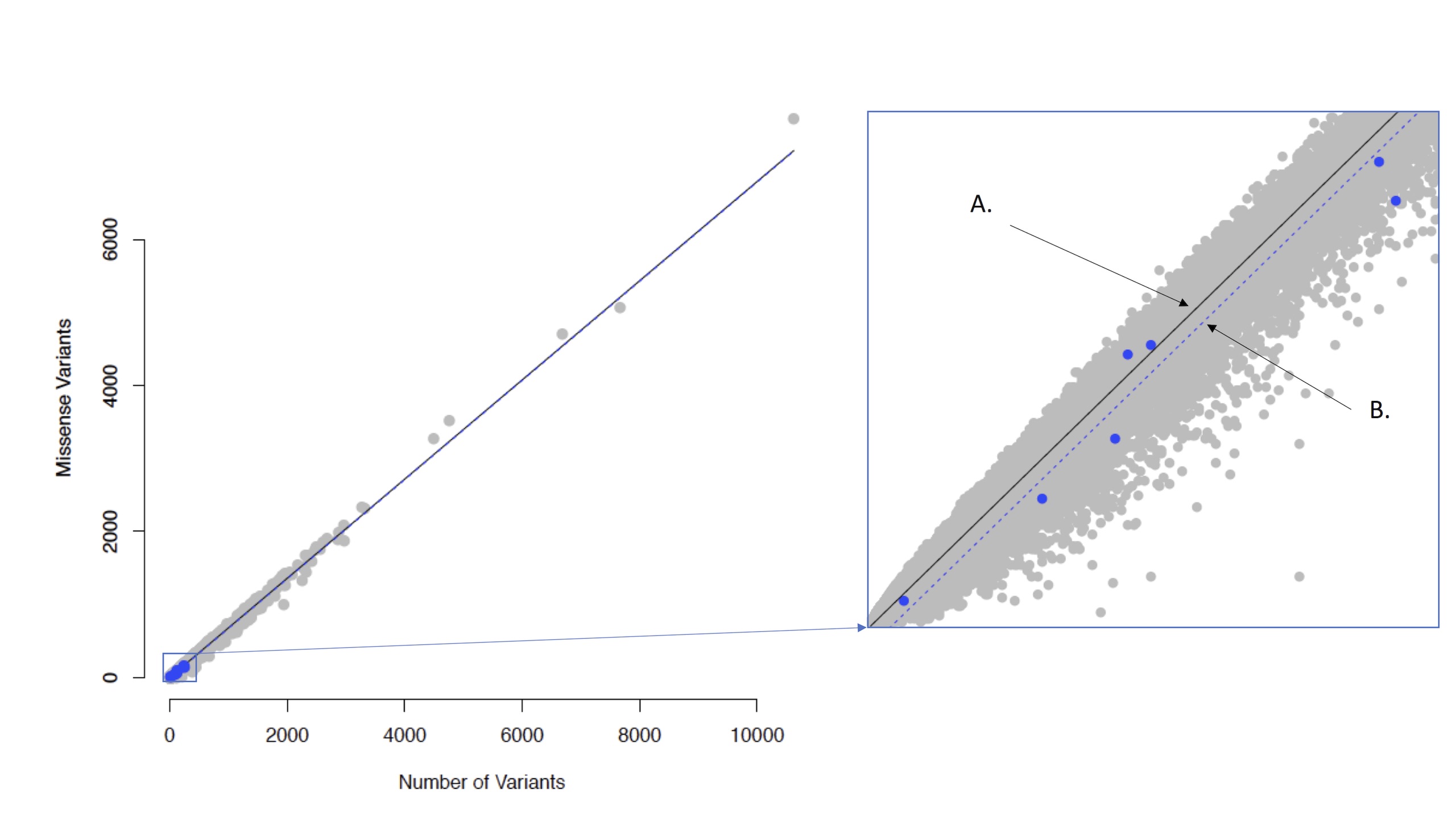
Localized Intolerance Model using Bayesian Regression (LIMBR) is a sub-regional (domains or exons) genic intolerance score. We fit a Bayesian hierarchical model explicitly characterizing depletion in functional variation at both the gene and sub-regional level. Figure 1 from our manuscript¹ depicts the approximate geometric interpretation of this approach, the model was regressed on missense variation versus all variation.

Data

The data on this website corresponds to our updated fit of the model on genome Aggregation Database (gnomAD) version v2.1 using 125,748 whole exome sequences. Two sets of scores are calculated by fitting different definitions of sub-regions across genes, once with genic sub-regions defined by exon boundaries and then again with sub-regions defined by functional domains, both using the Conserved Domain Database (CDD).^2,3 The filtered data from gnomAD first had to go through ‘PASS’ criteria, or in this version we also allowed for SEGDUP variants to be included, then further restricted to regions with at least 10x coverage in at least 70% of the samples. Additionally, any genes without any variation were excluded from the analysis.

Model

The number of missense variants within the ith sub-region of gene j, y_ij, as a function of the total number of variants within the ith sub-region of gene j, x_ij, through the following regression model,

y_ij = μ+α_j + α_i(j) + β₁x_ij + e_0ij,

We model α_j and α_i(j) as random effects within a Bayesian framework. We assume standard normal priors for α_j and α_i(j) but allow for separate prior variances for α_i(j) for each gene j. We begin by assuming an inverse gamma prior for the variances. Specifically, we choose α_j~N(0,σ² ) with hyper-parameters σ²~InvGamma( ϵ,ϵ) and ϵ~Uniform(δ,c), where δ is a small positive constant and c is a large positive constant to induce a diffuse prior. For the sub-region parameters, we use a similar structure but with a separate variance for each gene, i.e., we choose α_i(j)~N(0,σ_j² ) with hyper-parameters σ_j²~InvGamma( ϵ_j,ϵ_j) and ϵ_j~Uniform(δ,c). Note that by allowing for a gene-level variance, the α_ijs can be shrunken back to the gene level intolerance when there are no large differences between sub-region or when data is sparse. This will decrease the variability of the α_i(j)s, leading to more stable intolerance estimation.

To improve the ergodicity, α_i(j) was set to zero for genes with 2 or fewer sub-regions, this is effectively just collapsing genes with only 2 sub-regions eliminating any inflated within versus across chain variance. Further, it is known that the hierarchical model can be augmented, sometimes referred to as noncentral^4–6 or ancillary augmentation⁷, and similar methods are known to improve performance.^8,9 So, we introduced an additional hyper parameter v~N(0,1) for α^*_ij=vσ_j to reduce autocorrelation.

y_ij = μ+α_j + α^*_i(j) + β₁x_ij + e_0ij,

By introducing an auxiliary hyper parameter, the conditional variance structure is maintained while decoupling the random variables we wish to make inference on, Var(α_ij│σ_j² )=Var( α^*_i(j)│v,σ_j² ). The final score that is used for the analysis is the posterior mode of the combined genic and sub-region terms. The hierarchical model allows information to be shared across sub-regions, stabilizing intolerance estimates. A burn in of 1,000 with an additional 10,000 steps across 5 chains was run for both domains and exons.

For more details please see our article: Improved pathogenic variant localization via a hierarchical model of sub-regional intolerance

Reference

If you find the information or resources from this website useful in your research please cite our paper.

Hayeck, T. J., Stong, N., Wolock, C. J., Copeland, B., Kamalakaran, S., Goldstein, D. B., & Allen, A. S. (2019). Improved pathogenic variant localization via a hierarchical model of sub-regional intolerance. The American Journal of Human Genetics, 104(2), 299-309.

Bibliography

1. Hayeck, T. J. et al. Improved Pathogenic Variant Localization via a Hierarchical Model of Sub-regional Intolerance. Am. J. Hum. Genet. 1–11 (2019). doi:10.1016/j.ajhg.2018.12.020
2. Marchler-Bauer, A. et al. CDD: Conserved domains and protein three-dimensional structure. Nucleic Acids Res. 41, 348–352 (2013).
3. ... add the rest in XXX
4. Gussow, A. B., Petrovski, S., Wang, Q., Allen, A. S. & Goldstein, D. B. The intolerance to functional genetic variation of protein domains predicts the localization of pathogenic mutations within genes. Genome Biol. 17, 9 (2016).
5. Papaspiliopoulos, O. & Roberts, G. O. Non-Centered Parameterisations for Hierarchical Models and Data Augmentation. Bayesian Stat. 7, 307–326 (2003).
6. Papaspiliopoulos, O. & Roberts, G. Stability of the Gibbs sampler for Bayesian hierarchical models. Ann. Stat. 36, 95–117 (2008).
7. Betancourt, M. A General Metric for Riemannian Manifold Hamiltonian Monte Carlo. 327–334 (2013).
8. Yu, Y. & Meng, X.-L. To Center or Not to Center: That Is Not the Question—An Ancillarity–Sufficiency Interweaving Strategy (ASIS) for Boosting MCMC Efficiency. J. Comput. Graph. Stat. 20, 531–570 (2011).
9. Duan, L. L., Johndrow, J. E. & Dunson, D. B. Scaling up Data Augmentation MCMC via Calibration. (2017).
10. Liu, J. S. The collapsed Gibbs sampler with applications to a gene regulation problem. J. Amer. Stat. Assoc 89, 958–966 (1994).